Tweet Volume and Market Behavior

An Analysis of Tweets about Gold

July 2014

Introduction

The ability to monitor public commentaries about investments via Twitter naturally leads to many questions about correlations between tweets and asset price behavior. This study examines the relationship between the volume of tweets about gold and daily gold price returns as well as daily gold price volatility. The period under study is June 30, 2012 - June 30, 2014.

Tweets

Twitter's API provided a random sample of tweets that were authored by a select group of about 150 tweeters. These tweeters included media sources such as The Wall Street Journal, financial blogs such as Seeking Alpha and financial market commentators such as Keith McCullough. All tweets that occur from the previous day after 15:00 GMT, Day 1, to those that occur before 15:00 GMT on the next day, Day 2, are considered contemporaneous with the gold price fixing of Day 2. The logic is that any thoughts expressed after 15:00 GMT would be discounted in the closing price the following day.

The "gold_load.r" file reads the tweets provided by Twitter's API and filters out only those authored by the select group of tweeters. It then filters out those that mention "gold", "GLD", "IAU" or "precious metals". The dataframe "goldtweets" contains all of these tweets. From this set, tweets per day are calculated and put into dataframe "gtw".

source("gold_load.r")
goldtweets$date <- as.Date(substr(goldtweets$created_at,1,10))
goldtweets$n <- 1  # number of tweets per day
goldtweets <- as.data.table(goldtweets)
gtw <- goldtweets[ ,sum(n), by = date]

Summary of daily tweet data:

summary(gtw$V1)

##    Min. 1st Qu.  Median    Mean 3rd Qu.    Max. 
##     1.0    16.0    36.0    39.3    50.2   573.0

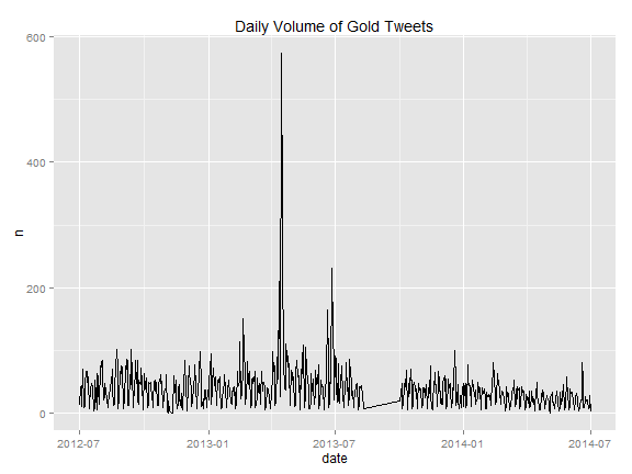
The graph below shows a large spike in tweets in April 2013 when the price of gold dropped sharply. The graph also shows a period of missing data, 8/10/2013- 10/3/2013.

qplot(date, V1, data = gtw, geom = "line", main = "Daily Volume of Gold Tweets",
      ylab = "n")

The tweet data needs to be grouped according to days which are trading days and days which are not trading days (weekends and holidays). New variables "tw" and "wtw" are created to differentiate between the two. The variable wtw contains the number of tweets sent during weekends and holidays and is assigned to the next date the market is open, typically a Monday. For all other days, the wtw variable is zero. The wtw variable and the tweet data for trading days are put into a new dataframe, "gt", which has only dates which are trading days.

tw <- gtw[gtw$date %in% p$date, ]
wtw <- as.data.frame(gtw[!(gtw$date %in% p$date), ])

#correcting for xmas and new year in wtw tallies
wtw$date <- as.character(wtw$date)
#2012 Market closed 12/22-12/26, 12/15 taken care of in next section
wtw[wtw$date == "2012-12-26",2] <- wtw[wtw$date == "2012-12-26",2] +
   wtw[wtw$date == "2012-12-24", 2] +  wtw[wtw$date == "2012-12-23", 2] +
   wtw[wtw$date == "2012-12-22", 2]
wtw <- wtw[!wtw$date == "2012-12-24" & !wtw$date == "2012-12-23" &
       !wtw$date == "2012-12-22", ]
#2012 Market closed 12/29-1/2, 12/31 taken care of in next section
wtw[wtw$date == "2013-01-01",2] <- wtw[wtw$date == "2013-01-01",2] +
   wtw[wtw$date == "2012-12-29", 2] +  wtw[wtw$date == "2012-12-30", 2]
wtw <- wtw[!wtw$date == "2012-12-29" & !wtw$date == "2012-12-30", ]

wtw[wtw$date == "2013-12-26",2] <- wtw[wtw$date == "2013-12-26",2] +
   wtw[wtw$date == "2013-12-24" , 2]
wtw <- wtw[!wtw$date == "2013-12-24", ]
#wtw[wtw$date == "2014-01-01",2] <- wtw[wtw$date == "2014-01-01",2] +
 #  wtw[wtw$date == "2013-12-31", 2]
#wtw <- wtw[!wtw$date == "2013-12-31", ]
wtw$date <- as.Date(wtw$date)

for(i in 1:nrow(wtw)){wtw[i,3] <- (wtw[i+1,1]-wtw[i,1])}
#correcting last observation
wtw[nrow(wtw),3] <- 6
for(i in 1:nrow(wtw)){
  if(wtw[i,3] > 1){
    wtw[i,4] <- wtw[i,1] + 1
  }else{
    wtw[i,4] <- wtw[i,1] + 2
  }
}
wtw[,1] <- as.Date(wtw[,4])
wtw <- wtw[,1:2]

wtwDateSum <- group_by(wtw, date)
wtw <- summarise(wtwDateSum, n = sum(V1))
# merge tweets and weekend tweets into gt
gt <- merge(tw,wtw, all = TRUE, by ='date')
setnames(gt,"V1", "tw")
setnames(gt,"n", "wtw")
gt[is.na(gt)]<- 0

Gold

The London afternoon gold price fixing, which occurs at 15:00 hrs GMT, is used as the reference price for gold. Gold price data comes from the World Gold Council (https://www.gold.org/research/gold-price-range-currencies-december-1978-xls-version). The "gold_load.r" file reads the gold price data and puts it into a dataframe "p".

From the price data, a time series with the daily gold returns is generated, "pdata". The dataframe "pdata.df" contains both the price returns and the absolute value of the returns

pdata <- as.xts(p$price,order.by = p$date, .RECLASS=TRUE)
pdata <- na.omit(Delt(pdata, x2 = NULL, k = 1, type = c("arithmetic", "log")) * 100)
#pdata is now class matrix with rownames NULL 
pdata.df <- as.data.frame(pdata, row.names = rownames(pdata), stringsAsFactors = FALSE)
colnames(pdata.df)[1] <- "r" #return variable
pdata.df$date <- as.Date(row.names(pdata.df))
pdata.df$ar <- abs(pdata.df[,1]) #volatility variable

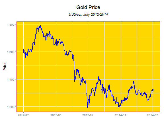
After a multi-year bull market, the price of gold corrected sharply in 2013, losing over 27% of its value in US Dollars. Gold suffered one of it's greatest single day price declines on April 15, 2013 when it lost over 9% of its value. In June 2013, gold reached its lowest price in recent history, $1,192/oz.

#Gold Price Plot
plot.title = 'Gold Price'
plot.subtitle = 'US$/oz, July 2012-2014'
plot <- ggplot(p, aes(x=date, y=price)) +
  geom_line(colour = "blue",size = 1) +
  geom_hline(aes(yintercept=min(p$Price), col = "red"))+
  ylab("Price") + xlab(" ") +
  theme(plot.title = element_text(size = 18, colour = "black"),
       panel.background = element_rect(fill = 'gold', colour = 'red'))
  plot <- plot +  ggtitle(bquote(atop(.(plot.title), atop(italic(.(plot.subtitle)),
      "")))) + scale_y_continuous(labels = comma)
suppressMessages(plot)

Correlations

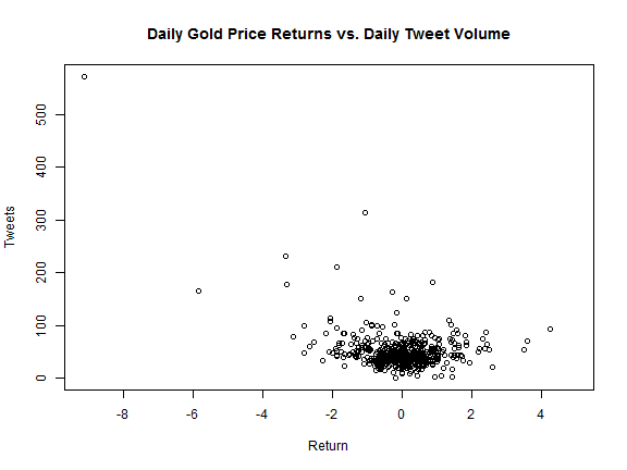
The graph below suggests a relationship between daily tweet volumes and daily returns

data <- merge(pdata.df,gt,by="date",all=TRUE) #dataframe "gt" merged with price data
plot(data$r, data$tw, main = "Daily Gold Price Returns vs. Daily Tweet Volume",
     xlab = "Return", ylab = "Tweets")

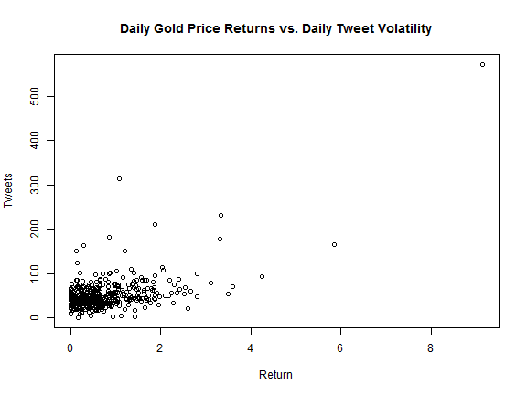
Also, the graph below suggests a relationship between daily tweet volumes and daily volatility

plot(data$ar, data$tw, main = "Daily Gold Price Returns vs. Daily Tweet Volatility",
     xlab = "Return", ylab = "Tweets")

The dataset is split into two groups, data1 and data2, due to a large gap in the time series data.

data1 <- data[data$date < as.Date("2013-08-10"),]
data1$tw <- na.approx(data1$tw) #fill in sporadic missing data
data1$wtw <- na.approx(data1$wtw) #fill in sporadic missing data
data2 <- data[data$date > as.Date("2013-10-03") & data$date < as.Date("2014-07-01"),]

In data1, the range of returns (r), volatility (ar), and tweet volumes (tw) is larger than in data2.

summary(data1[2:4])

##        r                ar              tw       
##  Min.   :-9.150   Min.   :0.000   Min.   :  0.0  
##  1st Qu.:-0.479   1st Qu.:0.200   1st Qu.: 40.0  
##  Median : 0.000   Median :0.450   Median : 50.0  
##  Mean   :-0.063   Mean   :0.735   Mean   : 58.9  
##  3rd Qu.: 0.446   3rd Qu.:0.985   3rd Qu.: 67.0  
##  Max.   : 4.262   Max.   :9.150   Max.   :573.0

summary(data2[2:4])

##        r                ar              tw     
##  Min.   :-2.816   Min.   :0.000   Min.   :  9  
##  1st Qu.:-0.558   1st Qu.:0.275   1st Qu.: 26  
##  Median : 0.076   Median :0.577   Median : 36  
##  Mean   : 0.004   Mean   :0.729   Mean   : 37  
##  3rd Qu.: 0.573   3rd Qu.:0.968   3rd Qu.: 44  
##  Max.   : 3.596   Max.   :3.596   Max.   :100

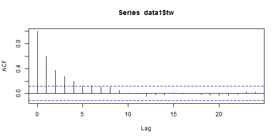
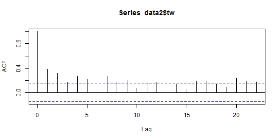
In both datasets tweets are autocorrelated

acf(data1$tw)

acf(data2$tw)

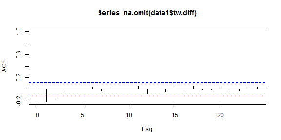
Differencing the tweets so that autocorrelation disappears:

data1$tw.diff <- c(NA,diff(data1$tw, lag = 1, differences = 1))
data2$tw.diff <- c(NA,diff(data2$tw, lag = 1, differences = 1))
acf(na.omit(data1$tw.diff))

acf(na.omit(data2$tw.diff))

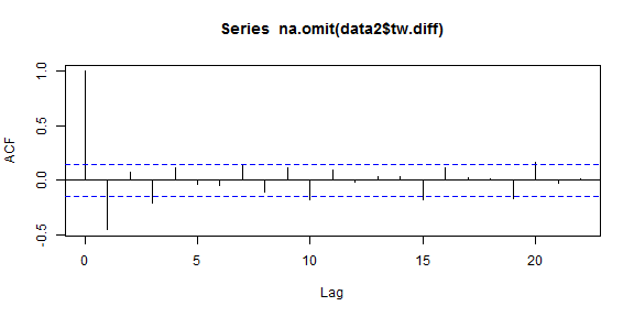
The series tw.diff is AR(1), so regressions of returns and volatility as a function of the change in tweets and the lagged value of change in tweets is a reasonable approach.

Tweet Volume and Daily Price Returns

An OLS regression of daily price returns as a function of the change in tweet volumes, same day and previous day, results in the following:

modR.data1 <- lm(r~tw.diff + lag(tw.diff), data1)
modR.data2  <- lm(r~tw.diff + lag(tw.diff), data2)
summary(modR.data1)

## 
## Call:
## lm(formula = r ~ tw.diff + lag(tw.diff), data = data1)
## 
## Residuals:
##    Min     1Q Median     3Q    Max 
## -4.107 -0.485 -0.047  0.512  3.195 
## 
## Coefficients:
##              Estimate Std. Error t value Pr(>|t|)    
## (Intercept)  -0.06846    0.05931   -1.15     0.25    
## tw.diff      -0.01474    0.00150   -9.82  < 2e-16 ***
## lag(tw.diff) -0.00807    0.00150   -5.37  1.6e-07 ***
## ---
## Signif. codes:  0 '***' 0.001 '**' 0.01 '*' 0.05 '.' 0.1 ' ' 1
## 
## Residual standard error: 0.998 on 280 degrees of freedom
##   (2 observations deleted due to missingness)
## Multiple R-squared:  0.278,	Adjusted R-squared:  0.273 
## F-statistic: 53.9 on 2 and 280 DF,  p-value: <2e-16

summary(modR.data2)

## 
## Call:
## lm(formula = r ~ tw.diff + lag(tw.diff), data = data2)
## 
## Residuals:
##    Min     1Q Median     3Q    Max 
## -2.854 -0.596  0.049  0.540  3.568 
## 
## Coefficients:
##               Estimate Std. Error t value Pr(>|t|)
## (Intercept)   0.000501   0.070611    0.01     0.99
## tw.diff      -0.001463   0.004863   -0.30     0.76
## lag(tw.diff) -0.003325   0.004865   -0.68     0.50
## 
## Residual standard error: 0.96 on 182 degrees of freedom
##   (2 observations deleted due to missingness)
## Multiple R-squared:  0.00256,	Adjusted R-squared:  -0.0084 
## F-statistic: 0.234 on 2 and 182 DF,  p-value: 0.792

The coefficients of the model for data1 are more significant than those for data2. Also, the p-values of the coefficients are smaller in the model for data1 than in the case of data2. The model for data2 does not allow us to negate the null hypothesis that the coefficient for the previous day's tweets is significantly different than zero.

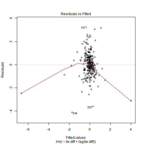
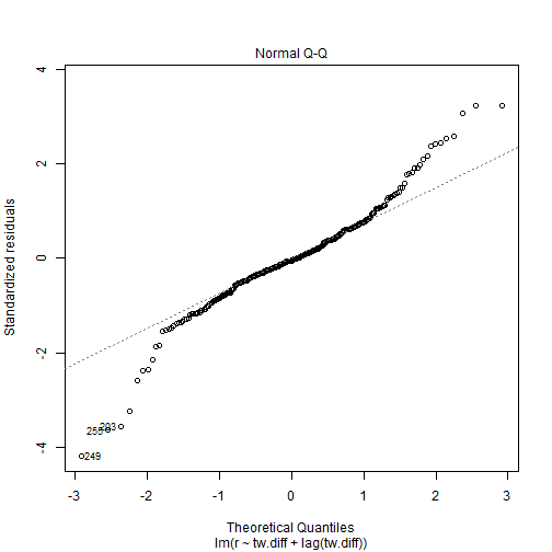
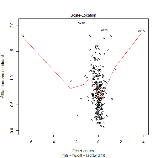
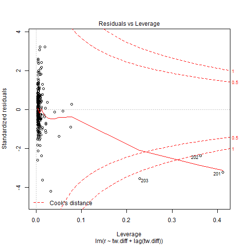
There seems to be some heteroscedasticity of the error terms in the model for data1, most likely because the model is having difficulty working with the observations with large negative returns/tweet volume. Heteroscedasticity does not seem to be a problem with data2.

plot(modR.data1)

plot(modR.data2)

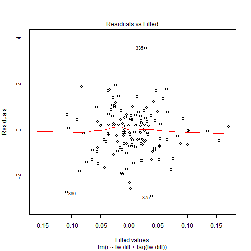
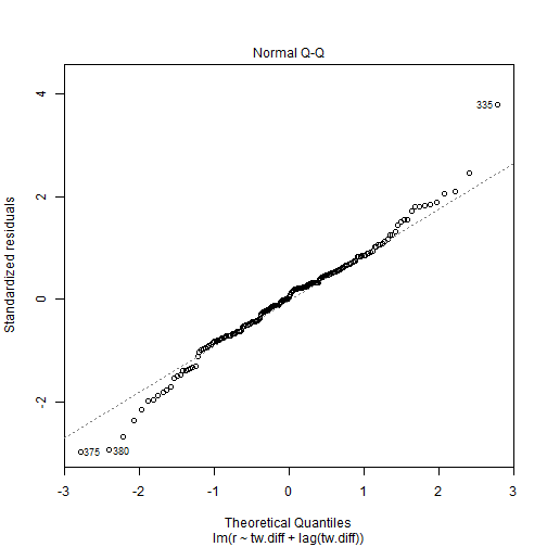
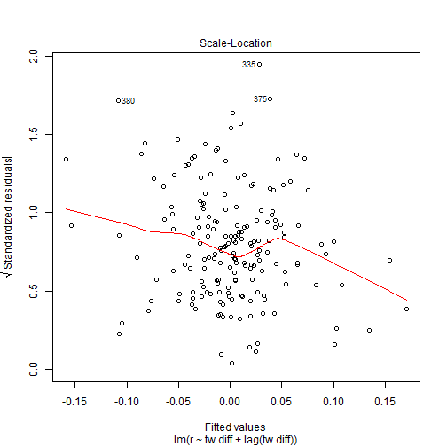
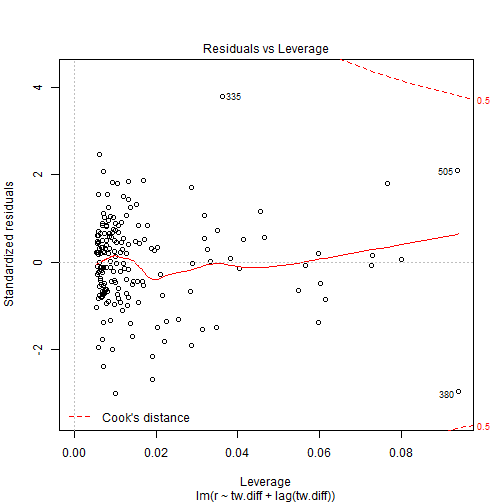
Using a robust covariance matrix estimator for data1 to test the coefficients of the model shows that the coefficient for the previous day's change in tweets is significant at the 10% confidence interval.

library(sandwich)
library(lmtest)
vcovHC(modR.data1)

##              (Intercept)   tw.diff lag(tw.diff)
## (Intercept)    3.839e-03 3.777e-05    1.476e-05
## tw.diff        3.777e-05 2.114e-05    1.077e-05
## lag(tw.diff)   1.476e-05 1.077e-05    1.731e-05

coeftest(modR.data1, vcov. = vcovHC)

## 
## t test of coefficients:
## 
##              Estimate Std. Error t value Pr(>|t|)   
## (Intercept)  -0.06846    0.06196   -1.10   0.2702   
## tw.diff      -0.01474    0.00460   -3.21   0.0015 **
## lag(tw.diff) -0.00807    0.00416   -1.94   0.0536 . 
## ---
## Signif. codes:  0 '***' 0.001 '**' 0.01 '*' 0.05 '.' 0.1 ' ' 1

Including the variable "wtw" (weekend and holiday tweets) does not seem to add explanatory value for the model for data1 but it does for data2 (at 5% confidence interval):

modRwtw.data1 <- lm(r~tw.diff + lag(tw.diff) + wtw, data1)
modRwtw.data2  <- lm(r~tw.diff + lag(tw.diff) + wtw, data2)
summary(modRwtw.data1)

## 
## Call:
## lm(formula = r ~ tw.diff + lag(tw.diff) + wtw, data = data1)
## 
## Residuals:
##    Min     1Q Median     3Q    Max 
## -4.047 -0.520 -0.023  0.496  3.079 
## 
## Coefficients:
##              Estimate Std. Error t value Pr(>|t|)    
## (Intercept)  -0.10418    0.06444   -1.62     0.11    
## tw.diff      -0.01496    0.00151   -9.93  < 2e-16 ***
## lag(tw.diff) -0.00810    0.00150   -5.40  1.4e-07 ***
## wtw           0.00570    0.00406    1.40     0.16    
## ---
## Signif. codes:  0 '***' 0.001 '**' 0.01 '*' 0.05 '.' 0.1 ' ' 1
## 
## Residual standard error: 0.996 on 279 degrees of freedom
##   (2 observations deleted due to missingness)
## Multiple R-squared:  0.283,	Adjusted R-squared:  0.275 
## F-statistic: 36.7 on 3 and 279 DF,  p-value: <2e-16

summary(modRwtw.data2)

## 
## Call:
## lm(formula = r ~ tw.diff + lag(tw.diff) + wtw, data = data2)
## 
## Residuals:
##    Min     1Q Median     3Q    Max 
## -2.770 -0.539 -0.021  0.554  3.637 
## 
## Coefficients:
##               Estimate Std. Error t value Pr(>|t|)  
## (Intercept)  -0.079766   0.076768   -1.04    0.300  
## tw.diff      -0.000729   0.004804   -0.15    0.880  
## lag(tw.diff) -0.002670   0.004804   -0.56    0.579  
## wtw           0.016135   0.006499    2.48    0.014 *
## ---
## Signif. codes:  0 '***' 0.001 '**' 0.01 '*' 0.05 '.' 0.1 ' ' 1
## 
## Residual standard error: 0.947 on 181 degrees of freedom
##   (2 observations deleted due to missingness)
## Multiple R-squared:  0.0354,	Adjusted R-squared:  0.0194 
## F-statistic: 2.22 on 3 and 181 DF,  p-value: 0.0879

Tweet Volume and Daily Price Volatility

OLS regressions of daily volatility as a function of the change in tweet volumes, same day and previous day, show that the change in the previous day's tweet volumes has significant coefficients. Furthermore, the difference between these coefficients data1 and data2 is small.

modV.data1 <- lm(ar~tw.diff + lag(tw.diff), data1)
modV.data2 <- lm(ar~tw.diff + lag(tw.diff), data2)
summary(modV.data1)

## 
## Call:
## lm(formula = ar ~ tw.diff + lag(tw.diff), data = data1)
## 
## Residuals:
##    Min     1Q Median     3Q    Max 
## -1.474 -0.474 -0.197  0.239  4.449 
## 
## Coefficients:
##              Estimate Std. Error t value Pr(>|t|)    
## (Intercept)   0.73386    0.04652   15.78   <2e-16 ***
## tw.diff       0.01165    0.00118    9.89   <2e-16 ***
## lag(tw.diff)  0.00530    0.00118    4.50    1e-05 ***
## ---
## Signif. codes:  0 '***' 0.001 '**' 0.01 '*' 0.05 '.' 0.1 ' ' 1
## 
## Residual standard error: 0.783 on 280 degrees of freedom
##   (2 observations deleted due to missingness)
## Multiple R-squared:  0.271,	Adjusted R-squared:  0.265 
## F-statistic: 51.9 on 2 and 280 DF,  p-value: <2e-16

summary(modV.data2)

## 
## Call:
## lm(formula = ar ~ tw.diff + lag(tw.diff), data = data2)
## 
## Residuals:
##     Min      1Q  Median      3Q     Max 
## -0.9459 -0.4019 -0.0917  0.1932  2.3603 
## 
## Coefficients:
##              Estimate Std. Error t value Pr(>|t|)    
## (Intercept)   0.73058    0.04164   17.55  < 2e-16 ***
## tw.diff       0.01724    0.00287    6.01  9.9e-09 ***
## lag(tw.diff)  0.00598    0.00287    2.08    0.039 *  
## ---
## Signif. codes:  0 '***' 0.001 '**' 0.01 '*' 0.05 '.' 0.1 ' ' 1
## 
## Residual standard error: 0.566 on 182 degrees of freedom
##   (2 observations deleted due to missingness)
## Multiple R-squared:  0.168,	Adjusted R-squared:  0.159 
## F-statistic: 18.3 on 2 and 182 DF,  p-value: 5.59e-08

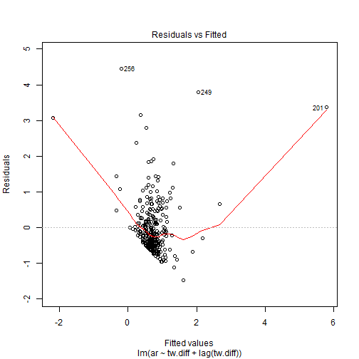
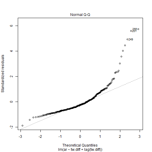
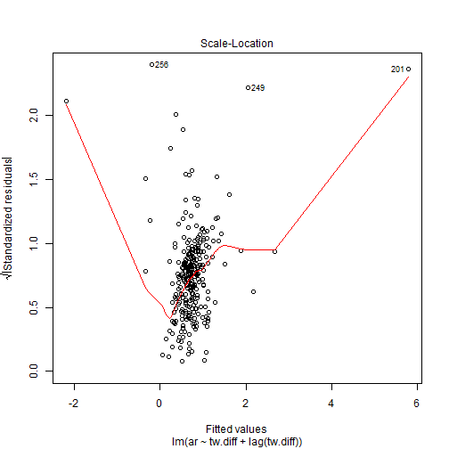
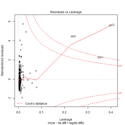
Again, there seems to be heteroscedasticity of the error terms in the model for data1, and less so for data2.

plot(modV.data1)

plot(modV.data2)

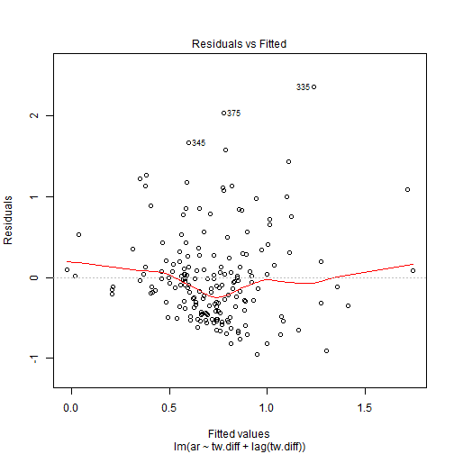
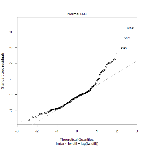
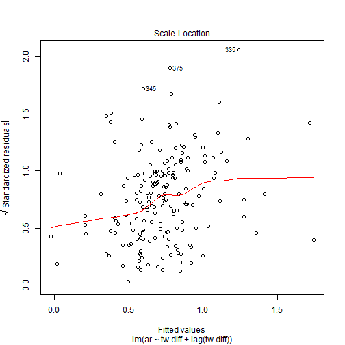
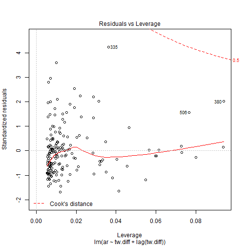
Using a robust covariance matrix estimator to test the coefficients of the models shows that the coefficient for the previous day's tweets is significant at the 5% confidence interval for data2, but not data1.

coeftest(modV.data1, vcov. = vcovHC)

## 
## t test of coefficients:
## 
##              Estimate Std. Error t value Pr(>|t|)    
## (Intercept)   0.73386    0.05075   14.46   <2e-16 ***
## tw.diff       0.01165    0.00568    2.05    0.041 *  
## lag(tw.diff)  0.00530    0.00434    1.22    0.224    
## ---
## Signif. codes:  0 '***' 0.001 '**' 0.01 '*' 0.05 '.' 0.1 ' ' 1

coeftest(modV.data2, vcov. = vcovHC)

## 
## t test of coefficients:
## 
##              Estimate Std. Error t value Pr(>|t|)    
## (Intercept)   0.73058    0.04220   17.31  < 2e-16 ***
## tw.diff       0.01724    0.00344    5.01  1.3e-06 ***
## lag(tw.diff)  0.00598    0.00281    2.13    0.035 *  
## ---
## Signif. codes:  0 '***' 0.001 '**' 0.01 '*' 0.05 '.' 0.1 ' ' 1

Including the variable "wtw" (weekend and holiday tweets) adds some explanatory value for data1 but not for data2:

modVwtw.data1 <- lm(ar~tw.diff + lag(tw.diff) + wtw, data1)
modVwtw.data2  <- lm(ar~tw.diff + lag(tw.diff) + wtw, data2)
summary(modVwtw.data1)

## 
## Call:
## lm(formula = ar ~ tw.diff + lag(tw.diff) + wtw, data = data1)
## 
## Residuals:
##    Min     1Q Median     3Q    Max 
## -1.407 -0.465 -0.210  0.255  4.088 
## 
## Coefficients:
##              Estimate Std. Error t value Pr(>|t|)    
## (Intercept)   0.68661    0.05021   13.67   <2e-16 ***
## tw.diff       0.01136    0.00117    9.68   <2e-16 ***
## lag(tw.diff)  0.00525    0.00117    4.49    1e-05 ***
## wtw           0.00754    0.00316    2.38    0.018 *  
## ---
## Signif. codes:  0 '***' 0.001 '**' 0.01 '*' 0.05 '.' 0.1 ' ' 1
## 
## Residual standard error: 0.776 on 279 degrees of freedom
##   (2 observations deleted due to missingness)
## Multiple R-squared:  0.285,	Adjusted R-squared:  0.277 
## F-statistic: 37.1 on 3 and 279 DF,  p-value: <2e-16

summary(modVwtw.data2)

## 
## Call:
## lm(formula = ar ~ tw.diff + lag(tw.diff) + wtw, data = data2)
## 
## Residuals:
##     Min      1Q  Median      3Q     Max 
## -0.9587 -0.3936 -0.0927  0.2033  2.3678 
## 
## Coefficients:
##              Estimate Std. Error t value Pr(>|t|)    
## (Intercept)   0.72179    0.04601   15.69  < 2e-16 ***
## tw.diff       0.01732    0.00288    6.01  9.8e-09 ***
## lag(tw.diff)  0.00605    0.00288    2.10    0.037 *  
## wtw           0.00177    0.00389    0.45    0.650    
## ---
## Signif. codes:  0 '***' 0.001 '**' 0.01 '*' 0.05 '.' 0.1 ' ' 1
## 
## Residual standard error: 0.568 on 181 degrees of freedom
##   (2 observations deleted due to missingness)
## Multiple R-squared:  0.169,	Adjusted R-squared:  0.155 
## F-statistic: 12.2 on 3 and 181 DF,  p-value: 2.51e-07

Conclusion

In this dataset, the change in tweet volumes was not a leading indicator of daily price returns. But the change in tweet volumes did show some indications of being a leading indicator of daily price volatility. The addition of weekend and holiday tweet volumes did not help predict either daily returns or volatility.